Navigation

Previous
Next
Homepage
FAQ
What's new
Sitemap

Topics

Introduction
Basic commands
Presentation
Page layout and printing
Functions
Copy, Paste and
relative and absolute references
Charts (graphics)
Macro commands
Analysis tools
Comments
Data list
Pivot table
Exercise: creating a model
Quiz

Tutorials

Word
Excel

Excel 2007/2010/2013
PowerPoint
Access

Others

Demonstration files
Texte en français

Contact

By e-mail
Join our Newsletter

Excel - Data lists

Introduction
Sort the data
Filters

• Automatic filter
• Advanced filter

The grid
Database functions

Introduction

Even if Excel is a spreadsheet, it offers you several tools to manage a small database. The term used in Excel is a data list. You can enter, change and remove data. The software offers also options to quickly find the data that you wish. There are also functions to analyze the mass of data that you accumulated. This Web page will give you an introduction to the lists of data and how to use the operations mentioned above.

The data, the fields and the records. Here are some terms that you should get acquainted.

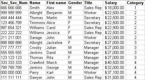
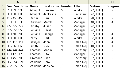
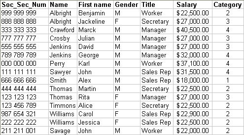
You can rewrite the data below in a worksheet or use this datalist.xls file. You can also find other files on the demonstration files Web page.

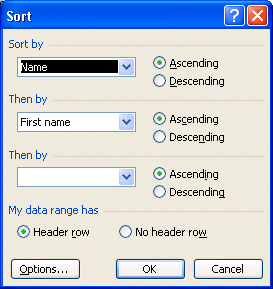
Here is a data list from employees of a company. As for the previous picture, the first row of a data list always contains the name of fields. Every following row contains a record that describes a person, a thing or an event according to the fields that you chose. A list of data should never have of empty rows. That is that all the records should follow itself continuously.

Sort the data

Excel allows you to sort out quickly the contents of a data list to help you to find quickly what you look for, to put of the order and to organize the data.

You can use buttons on the toolbar to sort out a column in increasing or lessening order. All the records of the data list will move according to the order that you chose. It's however necessary to pay attention not to make a block and then to sort out. Otherwise, only the data and not record will be sorted out. It will have the effect of mixing the data. Not recommended.

Excel offers you another way more advanced to sort out the data list. The next exercise consists in sorting out the records according to the name and the First name.

Place the cursor on any cell of the data list.
From the Data menu, select the Sort option.

You can sort out up to three fields at the same time in increasing or lessening order.

For the first sorting, select the Name field.
Sort in ascending order.
For the second sort field, select the First name field.
Sort in ascending order.

The sorting of the first box will have the priority on the second sorting. It means that Excel is first going to sort out on the name. For the records with the same name, Excel will sort out these records according to their First names.

Press the Options button.

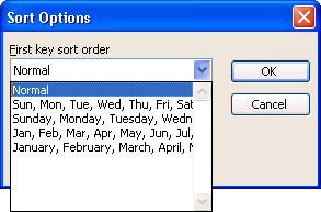
This is just for demonstrating you that you can sort out according to the normal order or according to the list that you prepared in advance.

Press the Cancel button.

To carry out the sorting, press the OK button.

The data list is now sorted out according to the chosen criteria. You can carry out a sorting up to three fields at the same time.

Filters

It can be frustrating to try to find data you need in a long data list. The automatic filter is an option to help you to find quickly the wished data.

The automatic filter

Place the cursor on any cell of the data list.
From the Data menu, select the options Filter and AutoFilter.

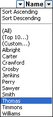
In the first row of the data list, there are now boxes of selection having the name of fields. By clicking the button in the right-hand side of the name of the field, you can limit what's shown in the list in what you need.

From the box of selection of the Name field, select Bibeau.

As you can notice, there's only two records, or persons in this case, who answers to the filter. It's always possible to combine filters to limit even more the results.

From the box of selection of the Titles field, select the Manager option.

From the Data menu, select the options Filter and Show All.
OR
From the filter boxes on the fields Name and Title, select the All option.

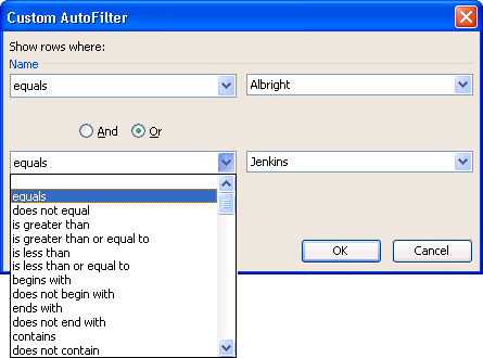
You can do more with AutoFilter. You can filter a field on two conditions.

Place the cursor wherever on the column of the Name field.

From the filter box for the field Name, select the Custom option.

A new window opens offering you to place until two conditions. Furthermore, you can choose among several conditions the one that answers better your needs.

For the first box, select the condition equals.
For the second box, select the name Albright.

Between both conditions, select the Or option.

For the third box, select the condition equals.
For the fourth box, select the name Jenkins.

To filter according to these conditions, press the OK button.

The automatic filter allows you to realize interesting searches. But the advanced filter offers you some more of possibilities and flexibilities.

From the Data menu, select the options Filter and Show All .
OR
From the filter box on the Name field, (All) select the option.

The advanced filter

Excel allows you also to carry out more complex searches. You can choose the fields of your choice as the criteria and enter values. You can also use the conditions AND and OR under the format of a wire netting.

Before using an advanced filter, you need at least two things: a list of data and a area of criterion.

Add the following data in the appropriate cells.

The first row of the criteria area should contain the name of the fields that you need for the criteria. For this exercise, it's about fields Title and Category. pay attention to the spelling! If the name is not identical in the name of the field of the data list, Excel will not show you the result that you want.

The following rows include the criteria. By default, Excel presumes the sign =. For the example, Title = Adminitrateur. You can also use the other ways to estimate such as >, <, <=>, =, <. To apply the conditions AND and OR, you should use the wire netting of Excel. The criteria that are on the same row use the criterion AND. In the example, the third row of the area of criterion s to Title = Worker AND Category = 4. The criteria that are on different rows use the condition OR. It allows to have the result of several conditions at the same time. For this exercise, all the criteria s to Title = Administrator OR Title = Worker AND Category = 4.

Place the cursor on one of the cells of the data list.

Otherwise, Excel will not want to carry out the filter.

From the Data menu, select the options Filter and Advanced Filter.

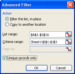
The advanced filter allows you two actions: filter the list or copy the data in another place. For the next stage, let the action filter. The following exercise will consist in using the copied action. Normally, Excel should have correctly chosen the good beach of cells for the data list. But, it's always necessary to verify. Contents in cells around the data list are not needed. It's as well necessary to make sure as Excel correctly chose the good criteria area. Otherwise...

Click in the Criteria range box.
Select a range of cells with the necessary cells for the criteria area. For the purpose of this exercise, select cells between I1 and J3.
Press the Enter key.

It's not necessary to take more cells than it's necessary for the criteria area. Otherwise, the result will not be what you expect.

Because there are the other actions to be carried out, press the OK button.

An advanced filter gives you more options than an automatic filter.

From the Data menu, select the options Filter and Show All.

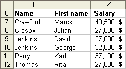
The advanced filter offers also another interesting option. Instead of masking the records that don't answer the criteria, the filter can copy "checks" records in another place on the worksheet. The next exercise consists in using the filter advanced with the option to copy the records.

Add the following data in the appropriate cells.

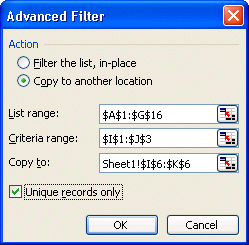
The first row of the destination of the advanced filter should contain the name of fields, correctly spelt, the result of that you want to see. Cells below these should be free. It's in those that the records that answer the criteria will be copied.

Place the cursor on one of the cells of the data list.
From the Data menu, select the options Filter and Advanced Filter.

From the list of the possible actions, select Copy to another location option.

The beach of the data list and the criteria area should be correct. But it's always necessary to verify. It remains to determine the destination.

Place the cursor in the Destination box.
Select cells with the names of the fields the result of that you want to see. For this exercise, select cells between I6 and K6.
Press the Enter key.
Activate the Unique records only option.

This last option avoids having the same record several times in the result if it answers several criteria that you entered.

Press the OK button.

Note:
Enlarge the salaries column if you see the "#" symbol.

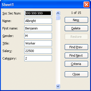
Excel copies the records in the place for that you asked.

The data form

Instead of entering, changeing and removing the data directly in the cells of a worksheet, Excel allows you to manage your lists of data by using a data menu. The next part consists in demonstrating you the functioning of this grid.

Place the cursor on one of the cells of the data list.
From the Data menu, select the Form option.

Excel offers you now the possibility of changeing the data of each of the records from this small form. Here is a short description of buttons.

The next exercises consist in putting into practice this menu.

Press the Find Next button.

The next record appears in the boxes of the left of the window. You can change their contents your choice. However, you can not change the contents of the field Category because it's about a formula.

By using the Previous and Next buttons, move through the records to change Josée Dupuis's salary from 22 500 $ to 24 500 $.

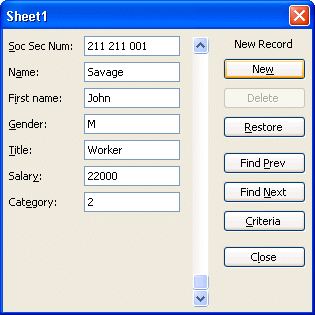
It's with regret that we learn that Mr. Paul Carter is leaving the company. Mr. John Savage was hired to replace him. Here are the relevant data to be added to the data list.

Place the cursor on one of the cells of the data list.
From the Data menu, select the Form option.

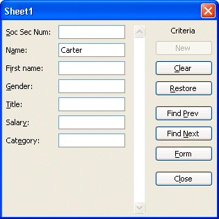
To accelerate the query, the option of the criteria will be used to look more quickly for the popular record.

Press the Criteria button.

Enter the text: Cardinal in the NAME box.
Press the Find Next button.

The record of Paul Cardinal will appear on the grid. It's now necessary to remove it from the data list.

Press the Delete button.

Excel asks you to confirm the deletion of the record.

Press the OK button.

It's now necessary to add the new employee.

Press the New button.

Enter the data in the appropriate cells.
Press the Enter key.
Press the Close button.

Mr Cardinal is not any more in the list and Mr Sauvageau was added to the end of the data list. As you notice it, it's easier to manage the data by using the bars that by looking on the worksheet.

The database functions

When you understood the lists of data and the areas of criteria, you can then carry out analyses with the available functions of Excel. There is 13 in everything. Here is a short description of some of these functions.

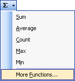
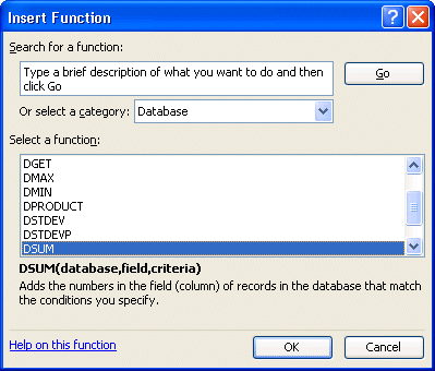
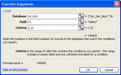
The next exercise consists in you demonstrating how to use these functions with =dbsum(). It's a question of knowing that's the total payroll of the administrators and the workers of category 4. The data list, A1 to G16, and the criteria area, I1 to J3, was already established in the previous exercises.

To use the function =dbsum(), and most of the others, you need three data or parameters: the area of the data list, the name of the field to be added and the area of the criteria area. Here is how to write it by using the assistant of the functions.

Place the cursor in the I4 cell.
From the toolbar, press the button .
OR
From the Insert menu, select the Function option.

The first column describes the categories of functions covered by Excel. The second column contains the list of the functions that you can use.

From the list of the categories of functions, select the Database option.
From the list of the functions, select DSUM.
Press the OK button.

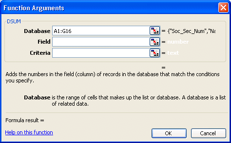
A new window appears asking you for the three parameters mentioned before. At the foot of this one, there is a description of the elements that you should enter each of the boxes. The first box is for the data list.

Click in the Database box.
OR
Press the button in the right-hand side of the Data base box.

Select the A1 to G16 cells.
Press the Enter key or the button at the end of the box as the box may be.

The cursor returns to the window of description of the function =databaseSum ().

Click on the Field box.

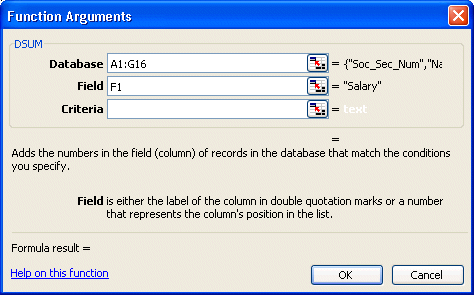
Notice that the description at the foot of the window looks now of the data for second box. You can also press the button to fetch the required data.

Click in the F1 cell.
Press the Enter key.

For the name of the field, you can enter the name of the field between quotation marks ("salary") or to enter the number of the column. Because the field salary is the sixth column of the data list, you can also enter the number 6.

All the required data entered. You have even the result at the foot of the window.

Press the OK button.

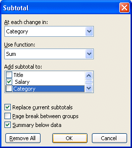
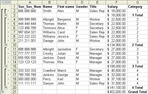
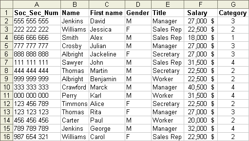
The result is 185 000 $. If you look at the contents of the bar of formula, you'll see that the formula looks like in =dsum(A1:G16; F1; I1:J3). It would work as well under this format =dsum(A1:G16; 6; I1:J3) or =dsum(A1:G16; "salary"; I1:J3). There are several ways to describe the field to be added. try now with the other functions of the category.

Analysis on groups

The functions of analyses can take out you interesting data. However, it can take time if you want the same data for several groups of data. For example, you need several functions to know the payroll by category of employees. Excel offers you the possibility of showing quickly subtotals of several functions (sum, averages...) by group.

Before even beginning analyses, it's first necessary to sort out the records on the field the subtotals of that you want to see. For this exercise, you must sort out on the field Category.

Category places the cursor on one of the records under the field.
By using buttons , to sort out in increasing order the field Category.

Here is what should look like data list if you completed all the operations of this Web page. It's now the time to see the total of salaries by category.

Place the cursor on a cell of the data list.
From the Data menu, select the option Sub-totals.

From the first box, Category selects the field.
For the second box, select that you want the Sum function.
From the third box, select that you want the sum the Salary field.

The window of the subtotals offers you also the possibility of replacing the total under of previous analyses. You can also accumulate these analyses to have more data. For example, you can have the sum and the average at the same time on the worksheet. It's necessary to pay attention to the function NBVal that's supposed to give the number of record by group. However, it does not seem to want to work correctly with the other functions.

You can also ask to have a page break after every group. This is interesting if you think of printing the results. You can also have at the end of the list of data a synthesis of the functions for that you asked.

Press the OK button.

The options to the left of the worksheet allow you to mask (-) and of rafficher (+) the categories. You can then concentrate the elements that you consider important. Buttons 1, 2 and 3 allow to mask and to show the synthesis, the subtotals and the records. Press these buttons to see their effects.

To return to the initial presentation:

Place the cursor on a cell of the data list.
From the Data menu, select the Sub-totals option.
Press the Delete all button.

The list reappears without the sums of the categories. You can now push your analyses a little farther thanks to the data list and the options.