 |
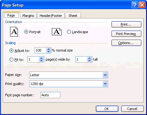
Under the Page tab, in the section Orientation, Excel asks you for the orientation of the pages to print.
In the scaling sections, you can manually
change the size of your spreadsheet by reducing or increasing it. This is very practical when all the columns of you're worksheet should be on one page only. You can also ask Excel to find automatically the best size to enter your document
on to X pages in widths and Y pages in height. At any time, you can look at
the printout before printing by pressing the review button. You can also change
the type of paper (letter size, legal, newspaper ...) as well as the quality
of the printing. For printing in the computer lab, be sure that the paper size
is always " US Letter ". The last option allows you to choose the page number
that will begin the printout. For example, the first page of your printout could
be numbered page 5 and so on. |
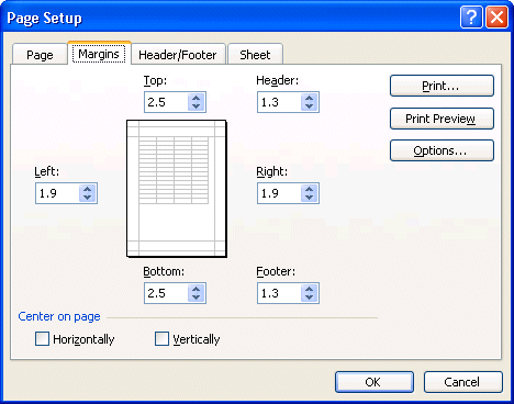 |
Under the Margins tab, you can determine the margins, the width between
the border of the page and your text, for the file as well as those for the
header and the footer of the page. You can also choose to center horizontally
and vertically your worksheet on the page. You can also determine the place
for the header and the footer for the worksheet your about to print. The outline
in the middle of the window gives you an idea of the effect of these choices
on the paper. |
|
Under the Header/Footer tab, you can determine what will be in the header
and the footer of each of the pages of the printout. If you don't want a header
or a footer, select the first option, "none", from the list of the
predetermined options. |
Personalize the header and footer.
It's sometimes
useful
to add a header or a footer to a document. It helps to
identify the document and what it's supposed to represent. For example, a header
with the title "Monthly revenues and expenses for May 2006" says it
all. The next exercise consists in writing the name of the document, your name,
as well as the date and the hour of the printout.
 Under
the Header/Footer tab, press the Custom Header button. Under
the Header/Footer tab, press the Custom Header button.
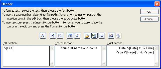
The options to personalize the header will appear as above. They are the same
options as for the page footer. In the middle of the window, there is a series
of buttons. They are the options most often used. The section at the bottom is separated
into three boxes. The left box will contain the text that will be written on
the left side of the page. The box in the middle will contain the text that
will be in the middle of the header and so on.
Click
in the left box.
Press
the  button
to insert the name of the file. button
to insert the name of the file.
Click
in the box of the middle.
Write
your first name and name.
Click
in the box of the right-hand side.
Write: Date: and press the  and and buttons. buttons.
The current date and time and the time of the printout will appear on the right
side of the header.
Press
the Enter key.
You can write many rows in a header or footer. The next part consists of
adding the page number and the total of pages in your printout.
Write Page and press the  button. button.
Write of and press the  button. button.
Press
the OK button.
Press
the Preview button
Press
the zoom button to better see the header.
The result should look like this.

The last exercise demonstrated how you can use the options by adding text and/or combining them to give a better results. It's also possible to write as
many rows as you need in the header or footer.
Press
the Close button to return to the page layout options.
Click
on the Sheet tab.
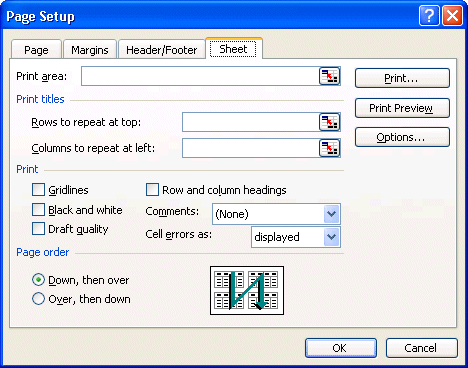
Under the Sheet tab, in the print area section you can determine what range of cells will be printed
in the printing area box. You can determine the area you want to print. Instead of printing all the contents of a worksheet, you can choose
to print only a part of it.
The titles boxes are very practicalin a worksheet. Often, you use the first rows and the
first columns in a worksheet to write the important titles such as: income,
charges, gross profit,etc, the months,etc. These titles will not print on the second
page or the following pages unless you force Excel to make it so. The option Print titles will reprint the selected rows and columns on to every page. Be careful, not
to put these rows and columns in the printing area. Otherwise, they are going
to be printed twice on the first page of your printout.
You also have access to other options:to print the grid on all the pages,
to print in black or white or in "draft" mode. It's also possible
to print the rows and columns headings (A, B, C, 1 , 2 , 3...) and even your
comments.
The printing area
Besides allowing you to print your entire spreadsheet, Excel allows you to
print a part of your worksheets. It's however necessary to determine in advance
the printing area that you need. There are several ways to carry out this task.
From
the File menu, select the Printing area and Define options.
Make
a range of cells with the area that you need to print.
OR
From
the File menu, select the Page Setup option.
Select
the Sheet tab.
Click
in the Print area box.
Select
the range of cells that you need to print.
While pressing on theCTRL key, you can select
several areas to print at the same time. However, every area will be printed
on a different page.
Printing
If you press the  button, Excel will print all the contents of the worksheet shown on the screen or
according to the options that you have chosen in the page layout. You can however control some options for printing. The next part explains
these options. button, Excel will print all the contents of the worksheet shown on the screen or
according to the options that you have chosen in the page layout. You can however control some options for printing. The next part explains
these options.
From the File menu, select the Print option.
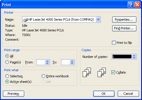 |
The window offers you several options. In the Printer section, you can choose the
type of printer on which your document will be printed. If you work in an office,
it may be possible that you have access to more than one printer. For example,
you could have access to a laser, ink jet printer or even a color printer.
In the Print range section, you have the options to print your entire document or only some pages
of you're file. file. This is very practical when you need to reprint a few
pages after a correction.
In the Print what section, Excel offers you to print the
block that you selected first, to print the worksheet where the cursor
is located or to print all the worksheets of your file that contains a number, text
or a formula. |
In the Copies section you can choose the number of copies that
Excel will print.
Page break
The previous sections showed you how to change the presentation
of the document on paper and the options for printing. But what if you wanted
a part of the document to always be at the start of a new page? Excel offers
you the possibility of putting in page breaks at any place in a worksheet. The
next part of this page demonstrates how to use page breaks.
Place
the cursor in the B2 cell.
From
the Insert menu, select the Page break option.
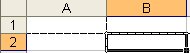
The page break will be placed above and to the left of the active cell. The
dotted rows indicate the separation between pages to be printed.
To remove a page break.
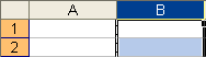
Place
the cursor in the cell in the intersection of the page breaks. For the exercise,
place the cursor in the B3 cell.
From
the Insert menu, select the option Delete Page Break.
In that box, the vertical page break will be deleted but not the horizontal
page break. The B3 cell was only tied to the vertical page break. Any
cell in the B column, apart from B2, would be able to delete the
vertical page break. The B2 cell could erase both vertical and horizontal
page breaks.
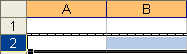
Place
the cursor in the B2 cell and delete the horizontal page break.
To insert only a vertical page break.
Click
on the letter of the column that you want to insert the page break. For the
exercise, select the B column.
From
the Insert menu, select the Page break option.
The page break will be placed on the left-hand side of the selected column.
Delete
the page break.
To insert a horizontal page break.
Click
on the number of the row that you want to insert the page break. For the exercise,
select row 2 by pressing on the grey box with the number 2.
From
the Insert menu, select the Page break option.
The page break will be placed above the selected row.
Delete
the page break.
Outline of page breaks
The preview of the page breaks option showes you what the document will look like
on paper. But before, you must prepare the worksheet by entering some numbers
and a page break.
Enter
the number 1 in the A1 cell.
Enter
the number 2 in the B2 cell.
Enter
the number 3 in the C3 cell.
Enter
the number 4 in the D4 cell.
Enter
the number 5 in the E5 cell.
Enter
the number 6 in the F6 cell.
Place
the cursor in the C3 cell.
From
the Insert menu, select the Page break option.
From
the View menu, select the Page break preview option.
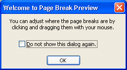
Excel gives you a message to inform you that you may move the page
breaks to better answer your needs.
If
you don't want to see this message anymore, click in box in the window and press
the OK button.
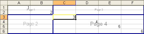
Excel will show you the worksheet by indicating the contents of the pages and
where the page breaks will appear. You can move the page break by placing the pointer
on them, pressing and holding the left mouse button and moving it around.
To
deactivate the option and return to the normal presentation, of the View menu, select the Normal option. |