Excel 2007 - Add a second axis to a chart

On occasion, it is better to present a data series on a second axis. The reason is because of the difference in scale between two data series or more. This page will show you comment to activate a secondary axis for your charts.

Select the range of cells from A1 to D4.

The Market share data series will be added later.

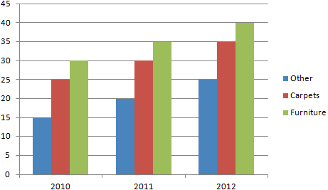
From the Insert tab, select Column Chart and 2-D Clustered column.

This is what the chart should look like.

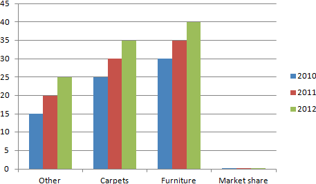
This is comment it would look if you added the market share data.

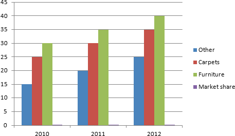
You can see that the axis have turned. The years are no longer on the X axis (horizontal). You could go to the Chart tools' Design tab and press the Switch Row/Column button to fix this. But there is another way to add data to a chart in Excel 2007/2010.

Select the range of cells from A5 to D5.
Press on the keys CTRL and C.
Click on the chart.
Press on the keys CTRL and V.

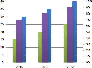
As you can see, it is hard to interpret the Market share data series even when you try to compare it to values ranging from 15 to 40. Imagine, comment hard it would be if the values where in the millions or more. In this case, adding a second axis from the Market share data is necessary. Here are the steps to activate it.

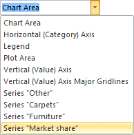
From the Chart tools' Layout or Format tabs, select the Series Market share.
Press the Format selection button.

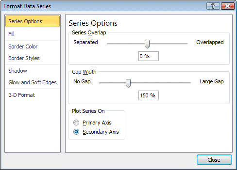
From the Series Options category, select Secondary Axis.
Press the Close button.

The secondary axis will appear on the right side of the chart. The values on it are in percentages compared to number on the axis on the left side of the chart. The problem in this present chart is that the Market share data series is now hiding the other values. The easiest way to settle this is to change the chart type for that data series.

Select the Market share data series.
From the Chart Tools' Design tab, press the Change Chart Type button.

From the Line category, select Line with Markers option.
Press the OK button.

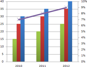
The Market share data series no longer hides the other data. The chart is easier to read and interpret. Within the Series Options, you can change whether a data series points towards the primary or secondary axis. Please inform your audiance which data series is using the primary or secondary data series.

You like what you read? Share it with your friends.

This site is hosted by 1&1.com