Excel 2010 - The Home tab

Microsoft Excel introduced a new menu structure called the Ribbon. All the commands are grouped under tabs. Each tab represents a step in creating a document. The Home tab represents the first step and is composed mostly of basic commands. This web page concentrates on explaining the commands under this tab.

You will find in the clipboard all the commands and options to cut, copy and paste objects. Since Office 2003, it can contain and manipulate many objects at the same time. It can also reproduce the formatting of a cell with Format painter.

The Cut option allows you to move an object from one location to another. You must select an object, cut it so that you can paste it elsewhere.

The Copy command allows you to select the element of your choice, leave it at the same location and paste it to as many other places. For example, you can recopy one or many formulas to many other cellsin your model. The border of the cells you selected to copy, or the source, will blink until you stop copying it. For example, the cell blinking will stop as soon as you go start to write in another cell.

The Paste command consists to placing the content of the cell, or range of cells, that you cut or copied into a new location. This option also offers many possibilities. They will be descripbed later in this text.

There is first the option is a basic Paste that will paste to the location of your choice the element that was cut or copied.

By pressing the second half of the Paste button, you will have access to all the possible options for this command.

This option allows you to copy only the formulas you cut or copied without taking into consideration the formatting such as the font style, its size and its background color.

This option will paste the value of the cell instead of copying the formula. For example, if the result of the formula =A1*A2 is 225, the Paste Values option will place the value 225 instead of the formula.

This option will paste the formula, the value and other presentation elements except the border.

The Transpose option consist of "turning" a range of cells on its side. Here is an example.

The Paste link option allows you to copy data located farther from the same worksheet, from another worksheet or from another workbook!

Excel will write the cell reference to view its content. In this case, the formula will be =$E$10.

This is a simple example. You can also make cell references coming from other worksheets in the same workbook. For example, paste link could also refer to =Sheet3!B25 which is the content cell B25 from the Sheet3 worksheet. The "!" is used to separate the name of the worksheet from the cell address.

The last paste link option is to copy the content of a cell from another workbook and to make a cell reference to it.

Open a new workbook.

Select the File tab.
Select New.
Select the Blank workbook option.
Press the Create button.
Place the cursor in the B5 cell.
Enter the value 500.

Select the File tab.
Select Save.
Save the workbook on your desktop under the name Link Example.

Copy the content of the B5 cell.
Return to the first worksheet.
Place the cursor in the A11 cell.

Press the arrow under the Paste button to view the options.
Select the option Paste link.

The reference in the cell will be ='[Link Example.xlsx]Sheet1'!$B$5. The name of the workbook is between brackets followed by name of the worksheet and the cell address. The link between the workbooks will remain active as long as the second workbook doesn't change location or change its name.

The next time you will open a file with a link to another worksheet, Excel will ask you if you want to activate the link between the files. It's a security mesure.

The next time that you will try to open this workbook, Excel will notice that there is a link to another Excel workbook.

Excel's security mesures will you ask you if you wish to active the link and retrieve the current value in the other workbook. This mesure is to make sure that you're not affected by viruses composed of macro commands.

The link to another workbook may have been changed if the document was moved or if its name changed. It will continue with the last known value available or check the connections to reestablish the link.

In this window, you will notice that the source of the link was not found. You can sever a link or change the source. This last option allows you to search thru your computer or your network to find the Excel workbook that you need.

Here is the list of all the options available options. You can decide to paste only a formula or it's resulting value, a comment that you have already written, a validation list (list of possible choices) and also of formatting. Another fun option is to paste one value by adding, subtracting, multiplying or dividing the value that is already in the cell. Here's a small example:

Enter the value 250 in cell A1.
Copy the content of cell A1.
Place the pointer over cell A1.
Select the option Paste special.
From the list of options, select Add.
Press the OK button.

Notice that the content of the cell is now 500, or the values 250 and added to the original 250. You can also use other mathematical operations (add, substract, multiply, divide) to create the results you want.

Format painter

Another interesting option that's not often used is to copy the formatting. It's very useful to recopy a presentation style or some conditional formatting. You created a title for a section of your model; selected the font, its size, color and other presentation options. Instead of reproducing each step, you can copy the formatting.

Write in the cell A1 cell the text: Title of the first section.
Write in the cell A3 cell the text: Title of the second section.
In the A1 cell, change the font size to 18 points and the text color to blue.
Place the cursor in the A1 cell.

From the Clipboard, select Format painter.

The presentation options of of this cell have been selected. You can now apply them to a cell or a range of cells.

Place the cursor in the A3 cell.

The formatting of the first cell will immediately be applied to the second. To reproduce the format to many cells, you must select the cell, or the range of cells, with the format of your choice, double-click for the Format painter button and apply it to all the cells of your choice. To stop, press once more on the Format painter button.

Like many commands, not all options are available on the screen; only the most popular ones. You can access more options by pressing the Dialog box launcher button located at the bottom right of each group of commands.

Press on the Dialog box laucher button for the clipboard.

This button will show or mask the task pane for the clipboard. When the clipboard is shown, you can cut and copy up to 24 elements. You only need to place the pointer in the cell of your choice and then press for the element to you wish to paste from the clipboard. You can also press for the Paste all button to paste all the elements of the clipboard in the order that they were included.

it's also possible of move, close or change the size the clipboard by pressing the button with the arrow to the right the clipboard title.

The Fonts group of commands allows you to choose the font, the size, put in bold, italic or underline, the border type and the cell's background color and pattern. These are the most often used options. Other options are available under the dialog box launcher.

Here is some more explications on these options.

The first box allows you to choose the font type for your text. The box will give you a preview of the font. The new Live preview option that came with Office 2007 allows you to view immediately the result even before you choose it.

This option determines the size of the font. You can change the size of the text at any time to better correspond with your needs.

Another way to change the size the text is to use the buttons increase or decrease the font size. The changement is immediate.

You can also place a border around a cell, or a range of cells, to improve your workbook's presentation. The options under the Border command will offer many options to determine the location, the border's thickness, the color and type of line for your borders. At the end of the list, the More Borders option will give you even more control on all the possible options.

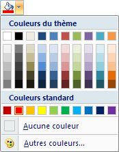This option allows you to determine the cell's fill color. From this window,you have access to 66 different colors. The More Colors option allows you to choose among more than 16 million colors.

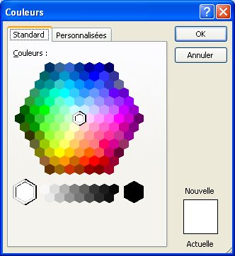
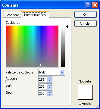
The standard tab offers a colors pallet with the most popular colors. The personalize tab gives you a precise control on the colors that you want. You can give one value of 0 to 255 to each basic color: red, green and blue. The total is 16 777 216 possible colors.

This option determines the color of the text that you written. You have access to the same options than the Fill colors described above.

From this tab, you can select the font type, its style and size, the type of underline, font color and some other attributes. You also have a preview box that will show you the results of your choices.

Once you're comfortable with your font choices, you can press the OK button. Otherwise, you can always press the Cancel button.

The alignment determines where the content of the cell will appear inside it. Will it be placed to the left, the center or the right side of the cell? You can add an indentation, a space between the cell border and the text, or change the text's orientation; put the text at an angle.

Excel doesn't limit to write your text horizontally. You can change the text's orientation to place some emphasis on the text or on a title.

Select the cell, or range of cells, that you want to change the text's orientation.
Select the one of the formatting options under the Orientation button.

Other orientation options are available under the Dialog box launcher button at the bottom right of this group of commands.

This determines the amount of space between the content and the cell's border. You can add more or less space between the text and the left cell border.

When the content of the cell is longer than the length of the cell, the text continues in the cell to the right if that cell is empty. Otherwise you will only see the leftmost section of the text. However, you can write as many rows of text in the same cell. The Wrap text option changes automatically the height of the cell so that you can see all the text that was entered. You can also use the combination of ALT and Enter keys to indicate where you want start writing on the next line.

An interesting option is to "merge" many cells together either in rows or columns into a single cell. It's very practical when you write a title that extends over many rows or columns.

You must view the options to master all the possible options. Those that have already used Excel 2003 or a previous version will be on familiar grounds. Except for a few changes to the presentation, you will find the same six tabs that where in previous versions of Excel. Experiment with these options and bring out a better presentation for your model.

Microsoft Excel offers many formatting styles for text, values and even for dates and times.

By pressing the arrow at the end of the box, you have a short list of available formats for values, text, dates and times. The last option, Other formats, allows you to choose among a greater formatting list and even to personalize to your own presentation style.

By selecting Other formats from the last menu, or by pressing the dialog box launcher box from Number group of commands, you will access all the possible formatting styles and options. The Personalize category allows you to add your own formats.

There are also the other tabs, identical from the Excel 2003 and previous versions that allows you to change the cell's formatting in many ways.

There are many possibilities under the Currency number format. Is it in dollars, in Euros, Yens or another denomination?

For other possibilities, select the More Accounting Formats.

From the Accounting category, you can choose among many more denominations than the ones mentioned in the previous list.

Allows to add or to remove decimal values from the formatting. Excel will round up the value according to the number of decimals that you want show.

You can also apply formatting styles to cells, a range of cells or to tables. The next section will give more information on how to use these options.

Conditional formatting gives you the option to change a cell's formatting (border, fill color, font color) when a condition is reached. For example, you could ask Excel to turn the cell red when a value turns negative or when the inventory for product reaches a critical level. You can apply many conditionnal formatting the same cell.

The conditional formatting options are elements of Excel that has been greatly improved with Excel 2007. Not, only does it allows you to change the formatting of a cell according to its value, but it allows you to realize some analysis on a range of values. This was only possible with specialized software before the arrival of Excel 2007.

Greater than: You can highlight the cells that have values above a limit that you determined.

Less than: You can highlight cells that have value below a certain limit.

Between: Highlight cells that are between a range of values.

Equal To: Highlight cells when its content is equal to a set value.

Text that contains: Highlight cells that contain some text.

A date occurring: Highlight cells that equals a set date or a range of dates (last week, last month ...)

Duplicate values: highlight cells that contain the same values or to unique values.

You can also manage the conditional formatting rules from this window. It even gives you another option to highlight according to a formula that you created. But, the result of that formula must either be TRUE or FALSE. So, your formula must start with the IF function and contain your formula in the criteria argument of the function. Ex. =IF(A5/B5>=5; TRUE;FALSE). You can create more complex formulas.

Highlight the top or bottom values from a range of cells. You can highlight the top/bottom 10 values, top/bottom 10%, values above or below average. Those are just the options available from this menu. You can have more control on what's highlighted by selecting the More Rules option.

This will return you to the Formatting Rule windows with the Format only top or bottom ranked values option selected. You can determine all the options including the cell's formatting for this new rule.

Not only can you read the values, but you also have a graphical representation of those values. It's easier to see which has the highest value or the lowest without having to read all the possible values

Increase the length of the column to better represent the data bar.

You can select a range of cells and apply color scales to them. The cell's background color will represent its value. In the color scale, the value at the bottom of the scale represents the lowest values. The color on top represents the highest values. You can also select the More Rules option to change how a color scale is applied.

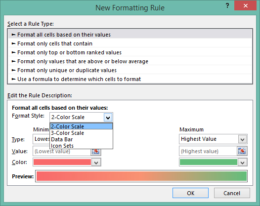From this window, you can apply a 2 or 3 color scale and choose the most appropriate colors for your values. With a 2 color scale, you select a color for the highest and lowest values. Excel will then create a color scale according to the colors you selected. With a 3 color scale, you can select a color for the top, bottom and median values.

You can also use a set of icons to represent a value. It will appear beside the value inside the cell. As you can see, there is a wide selection of icons to choose from. You can also select Other rules to determine how the icon set will be applied to the values.

You can be more selective on how the rules will be applied by selecting the More Rules option.

You can select the icon set of your choice and at what value should they change to the next icon. You can determine the change by selecting a number, a percentage, a percentile or according to a formula.

You can create your own conditionnal formatting rules to determine the type of formatting you want to use and how to apply it. You can also apply many rules to a single cell.

You can apply a cell style to a range of cells or to a table. You can quickly change how a worksheet is presented to your audience.

Creating a model is only the first part. You also need to adjust it to add or remove data from it. The next options allow you to manage your worksheet and your workbook. You can insert and remove cells, rows and columns by pressing just a few buttons. You can also format it to help its presentation.

You can insert and remove cells, rows and columns by pressing just a few buttons. At any time, you can add a cell, a row, a column in the worksheet. You can even add another worksheet if you need it.

This option can remove cells, rows or columns from the worksheet. This may be required to better organize your model.

Under the format option, you can adjust the length and height of a row or column. You can also mask them temporarily to better view values that are far apart in the worksheet or that you don't want other users to see.

You can also change the name on the worksheet's tab or ven its color. You can also protect the entire worksheet so that no user can change the values unless you unprotect some cell that you allow them to change.

With these commands, you can work on your worksheet to add formulas, fill in blanks or erase them, sort and filter a data list or search for content in your workbook.

Apart from the Sum function, you will have a list of the most recently used functions and access to all the other functions. To access even more functions, select More functions at the bottom of the list. This action will open the Insert Function dialog box. You will be able to search for the function you need from the list of all the functions Excel can provide.

Excel offers an Autofill option that you can use to fill cells with predetermined lists or from a range of values. The square on the bottom right of the active cell is the Autofill button. You must the cursor on the autofill button to activate the option. It can also be used to copy text, values or formulas.

At times, you need to remake a section of your worksheet. You can use the options of this section to clear out the content of the cells, it's formatting or comments.

Microsoft Excel has always had sort and filter options for data lists. This option is also available under the Data tab. This is where you will find all the instructions to use these options.

At times you need to change part of the data in your model. For example, a product changes name, a company changes address. You can use the options under the Find and Select commands to find and replace data, a cell references in your formulas, or even the content.